

Backpropagation and gradient descent: how AI learns
- Gabriel Gramicelli

- Apr 12, 2021
- 4 min read
Updated: May 5, 2021
Gradients and steepest descent
In the study of ANNs, we often aim to optimize a certain error/loss function. Doing so will increase model accuracy and achieve our goal. To do so, we must perform backpropagation, an algorithm first introduced by Paul Werbos in 1974. The process of optimisation means to either maximise or minimise the loss function, since we aim to decrease its error amount, we must minimise it. Methods such as newton’s method use the gradient of the function in order to determine the terrain around it and approach a local minimum. To do so, we must compute the definite gradient of the loss function with respect to each weight of our network, allowing us to determine the terrain near the gradient, and then find the direction of steepest descent (so we can minimise the loss function the fastest). The gradient in question can be computed as:
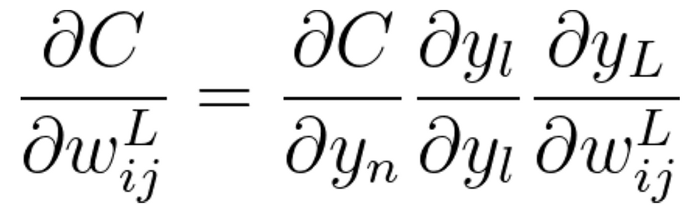
Where each y is a function that is influenced by the weight such that y^L is the first function using the weight. This simple multivariable chain rule can be used to find very nice gradient functions. Let’s find these.
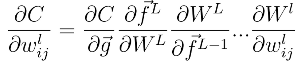
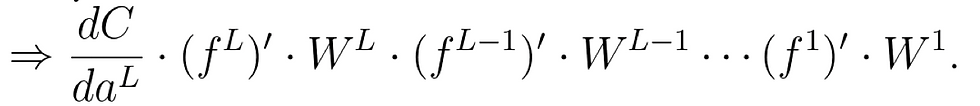
Now we are trying to find how a small nudge in a weight w affects the final C function. This means that we must calculate the gradient over all functions that apply w all the way to the final loss function. This gradient calculation can get very big over time, so we will use methods for optimising our compute costs. In general, A neural network can be written as:

where f^l is the activation function at layer l, B^l is the bias vector at layer l, W^l is the weight matrix at layer l, and V is the input vector. This means that to find the derivative the cost with respect to a weight:
Now this might seem standard at first, the derivative of the cost with respect to g is the sum of the derivatives of the operation done to each element (since the cost outputs a scalar value) with respect to that element, but how do we find derivatives that include matrices?
First, for a training set, the data will always be of the form:
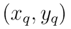
where x is an item and y is a label, and for backprop, we want to find the definite gradient at each pair. It is extremely inefficient to find the gradient only via chain rule since we are losing a chance of taking advantage of the linearity of our network, so we compute the gradient of each layer – specifically, the gradient of the weighted input of each layer, denoted by

Informally, the key point is that since the only way a weight in W affects the loss is through its effect on the next layer, and it does so linearly,
are the only data you need to compute the gradients of the weights at layer l, and then you can compute the previous layer and repeat recursively.
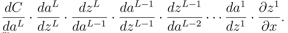
To compute the definite derivative at (x, y), we want the derivative of

, which denoting z as each layer’s input and a as each layer’s output is:
We may see:
Now since the transpose of a scalar is itself, we see that we can then find the derivative as:

, we can then introduce the auxiliary quantity
for the partial products (multiplying from right to left), interpreted as the "error at level l" and defined as the gradient of the input values at level l:

Now, this error is a vector, with equivalent size as of the vector of layer l. And since we go backwards in the network starting with the error vector at layer L,

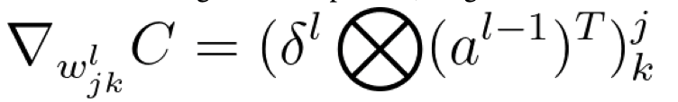
Thus, we can produce the gradient of the weights in layer l as:
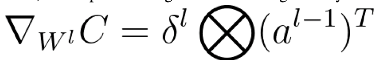
Since we are using the tensor product, we get that:
Ok, so we now have easily computable formulas for finding the gradients, and we should start to think of optimization methods. We must find the direction of steepest descent, so we can step in that direction and descend the quickest.
Let’s then look at a theorem that says the gradient vector is the direction of steepest descent:
Since we are trying to find what direction we can walk into in a high dimensional plane where the function is the cost function and the coordinates are the weights and biases, we wish that we may take a small step in each direction, and see the resulting step in the cost function (thus the partial derivative), then, we may call each of these directions to be vectors of length 1, such that the length does not affect the steepness. Thus, we can take the directional derivative and thus maximise:
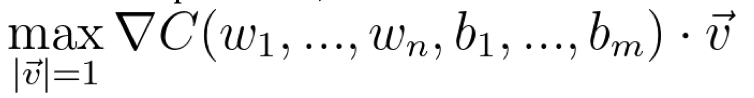
Since the dot product simply projects v onto nabla-C, we can see that the direction that maximises this equation is the very direction of nabla-C:
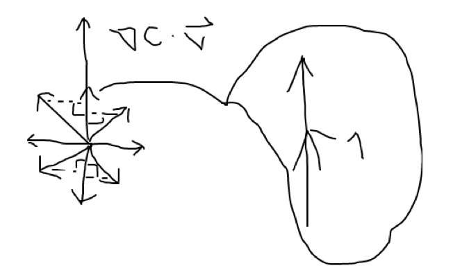
With this, we may confirm the formulas for finding the gradient and that the gradient is the very direction of steepest ascent (since we’ve maximised the function), meaning that the direction of steepest descent is the negative gradient.
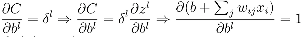
Lastly, the gradient of the bias may be computed as:
Optimisers and step
Now, we must figure out a way to walk in the direction of the steepest descent that is reasonable and functional. We may try to simply subtract the gradient from the weight/bias, yet this might result in large steps that may be as biased as the sample given. We may then apply a learning rate, a small quantity that may be 0.001 or so, to make each step tiny. We may even add some ‘history’ to create gradient descent:
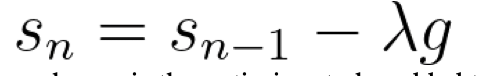
, where s is the optimiser to be added to the weight, lambda is the learning rate, and g is the gradient.


Comments